Recurrent Neural Networks
Motivation
Recurrent neural networks (RNNs) are typically used in sequence processing applications such as natural language processing and generation. Some specific examples include:
- Sequence classification: given a sequence input, produce a fixed sized output, e.g. determine the "sentiment" of a product review.
- Sequence generation: given a fixed sized input, produce a sequence output, e.g. automatic image captioning.
- Sequence tagging: given a sequence, produce a label for each token, e.g. part-of-speech tagging.
- Sequence-to-sequence mapping: given a sequence, produce another, not necessarily parallel, sequence. e.g. machine translation, speech recognition.
All feed-forward models we have seen so far (Linear, MLP, CNN) have a common limitation: They are memoryless, i.e. they apply the same computational steps to each instance without any memory of previous instances. Each output is obtained from the current input and model parameters using a fixed number of common operations:
A model with no memory is difficult to apply to variable sized inputs and outputs with nontrivial dependencies. Let us take sequence tagging as an example problem. To apply a feed-forward model to a sequence, one option is to treat each token of the sequence as an individual input:
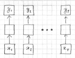
Applying the same computation to each input token makes sense only if the different input-output pairs are IID (independent and identically distributed). However the IID assumption is violated in typical sequence processing applications like language modeling and speech recognition where the output of one time step may depend on the inputs and outputs from other time steps.
Another option is to treat the whole sequence as a single input:
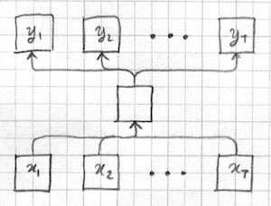
The first problem with this approach is that the inputs are of varying length. We could potentially address this issue using a convolutional architecture, and this is a viable alternative for sequence classification problems. However we have a more serious problem with variable length outputs: The space of possible outputs grow exponentially with length and output tokens have possible dependencies between them. Problems of this type are known as "structured prediction", see (Smith 2011) for a good introduction. It is not clear how to generate and score variable sized outputs in a single shot with a single feed-forward model.
Finally we can generate each output token separately, but take a fixed sized window around the corresponding input token to take into account more context:
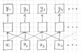
This is the approach taken by, e.g. n-gram language models, and Bengio's MLP language model. The problem with this approach is that we don't know how large the window needs to be. In fact different tokens may require different sized windows, e.g. long range dependencies between words in a sentence. RNNs provide a more elegant solution.
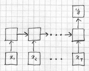
RNNs process the input sequence one token at a time. However, each output is not only a function of the current input, but some internal state determined by previous time steps:
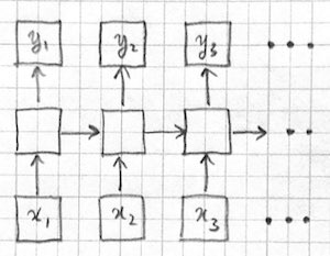
The state $h_t$ can be thought of as analogous to a memory device storing variables in a computer program. In fact, RNNs have been proven to be Turing complete machines (however see this and this for a discussion). At each time step, the RNN processes the current input $x_t$ using the "program" specified by parameters $w$ and the internal "variables" specified by $h_{t-1}$. The program stores new values in its internal variables with $h_t$ and possibly produces an output $\hat{y}_t$.
Architectures
Depending on the type of problem, we can deploy an RNNs with architectures other than the tagger architecture we saw above. Some examples are:
- Sequence classification
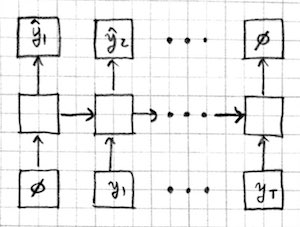
- Sequence generation
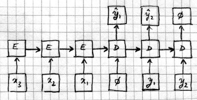
- Sequence to sequence mapping models which combine the previous two architectures. The input sequence is processed by an encoder RNN (E), and the output sequence is generated by a decoder RNN (D). Information is passed from the encoder to the decoder through the initial hidden state, or an extra input, or an attention mechanism.
julia function mlp1(w,x) h = tanh(w[1]x .+ w[2]) y = w[3]h .+ w[4] return y end
function rnn1(w,x,h) h = tanh(w[1]vcat(x,h) .+ w[2]) y = w[3]h .+ w[4] return (y,h) end
Note two crucial differences: First, RNN takes `h`, the hidden state
from the previous time step, in addition to the regular input
`x`. Second, it returns the new value of `h` in addition to the
regular output `y`.
## Backpropagation through time
RNNs can be trained using the same gradient based optimization
algorithms we use for feed-foward networks. This is best illustrated
with a picture of an RNN unrolled in time:
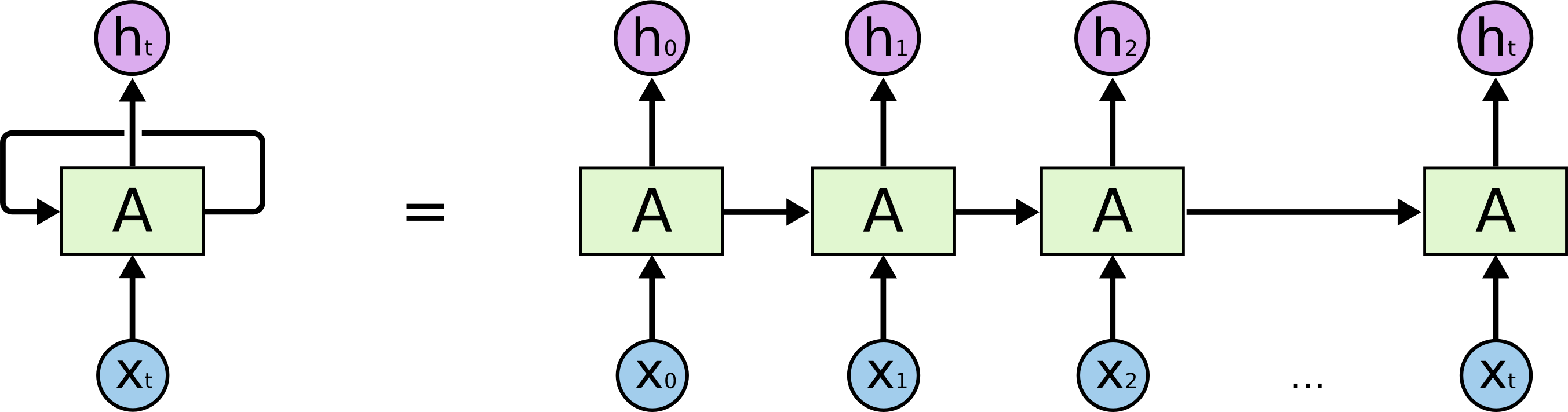
([image source](http://colah.github.io/posts/2015-08-Understanding-LSTMs))
The picture on the left depicts an RNN influencing its own hidden
state A while computing its output h for a single time step. The
equivalent picture on the right shows each time step as a separate
column with its own input, state and output. We need to keep in mind
that the *function* that goes from the input and the previous state to
the output and the next state is identical at each time step. Viewed
this way, there are no cycles in the computation graph and we can
treat the RNN as just a multi-layer feed-forward net which (i) has as
many layers as time steps, (ii) has weights shared between different
layers, and (iii) may have multiple inputs and outputs received and
produced at individual layers.
Backpropagation through time (BPTT) is the SGD algorithm applied to
RNNs unrolled in time. First, the RNN is run and its outputs are
collected for the whole sequence. Then the losses for all outputs are
calculated and summed. Finally the backward pass goes over the
computational graph for the whole sequence, accumulating the gradients
of each parameter coming from different time steps.
In practice, with Knet, all we have to do is to write a loss function
that computes the total loss for the whole sequence and use its
`grad(f)` for training. Here is an example for a sequence tagger:
julia function rnnloss(param,state,inputs,outputs) # inputs and outputs are sequences of the same length sumloss = 0 for t in 1:length(inputs) prediction,state = rnn1(param,inputs[t],state) sumloss += crossentropyloss(prediction,outputs[t]) end return sumloss end
rnngrad = grad(rnnloss)
train with our usual SGD procedure
[](Hinton 7b)
[](Unfolding picture)

## Vanishing and exploding gradients

RNNs can be difficult to train because gradients passed back through
many layers may vanish or explode. To see why, let us first look at
the evolution of the hidden state during the forward pass of an
RNN. We will ignore the input and the bias for simplicity:
julia h[t+1] = tanh(Wh[t]) = tanh(Wtanh(W*h[t-1])) = ...
No matter how many layers we go through, the forward `h` values will
remain in the `[-1,1]` range because of the squashing `tanh` function,
no problems here.  However, look at what happens in the backward pass:
julia dh[t] = W' * (dh[t+1] .* f(h[t+1]))
where `dh[t]` is the gradient of the loss with respect to `h[t]` and
`f` is some elementwise function whose outputs are in the `[-1,1]`
range (in the case of `tanh`, `f(x)=(1+x)*(1-x)`). The important thing
to notice is that the `dh` gradients keep getting multiplied by the
same matrix `W'` over and over again as we move backward, and the
backward pass is linear, i.e. there is no squashing function.

What happens if we keep multiplying a vector ``u`` with the same
matrix over and over again?  Suppose the matrix has an
eigendecomposition ``V\Lambda V^{-1}``.  After n multiplications in
effect we will have multiplied with ``V\Lambda^n V^{-1}`` where
``\Lambda`` is a diagonal matrix of eigenvalues. The components of the
gradient corresponding to eigenvalues greater than 1 will grow without
a bound and the components for eigenvalues less than 1 will shrink
towards zero. The gradient entries that grow without a bound
destabilize SGD, and the ones that shrink to zero pass no information
about the error back to the parameters.

There are several possible solutions to these problems:

* Initialize the weights to avoid eigenvalues that are too large or
  too small. Even initializing the weights from a model successfully
  trained on some other task may help start them in the right regime.
* Use gradient clipping: this is the practice of downscaling gradients
  if their norm is above a certain threshold to help stabilize SGD.
* Use better optimization algorithms: methods like Adam and Adagrad
  adjust the learning rate for each parameter based on the history of
  updates and may be less sensitive to vanishing and exploding
  gradients.
* Use RNN modules designed to preserve long range information: modules
  such as LSTM and GRU are designed to help information flow better
  across time steps and are detailed in the next section.

[](motivation: why do mlp rnns have a hard time learning? vanishing gradients relevant according to DL 10.7 are vanishing gradients only important for bptt? how does lstm solve them?)
[](Hinton 7d: why bptt is difficult, back pass linear.)
[](http://www.wildml.com/2015/10/recurrent-neural-network-tutorial-part-4-implementing-a-grulstm-rnn-with-python-and-theano/)
[](This may have a different math explanation: http://www.wildml.com/2015/10/recurrent-neural-networks-tutorial-part-3-backpropagation-through-time-and-vanishing-gradients/)
[](Adam and gclip DL 10.11)

## LSTM and GRU

[](lstm/gru: http://colah.github.io/posts/2015-08-Understanding-LSTMs/ DL 10.10)

The Long Short Term Memory (LSTM) and the Gated Recurrent Unit (GRU)
are two of the modules designed as building blocks for RNNs to address
vanishing gradients and better learn long term dependencies. These
units replace the simple `tanh` unit used in `rnn1`.

... To be continued
julia function lstm(weight,bias,hidden,cell,input) gates = hcat(input,hidden) * weight .+ bias h = size(hidden,2) forget = sigm(gates[:,1:h]) ingate = sigm(gates[:,1+h:2h]) outgate = sigm(gates[:,1+2h:3h]) change = tanh(gates[:,1+3h:end]) cell = cell .* forget + ingate .* change hidden = outgate .* tanh(cell) return (hidden,cell) end ```
Practical issues
input and output (word Embedding and prediction) layers
decoding and generating: greedy, beam, stochastic.
minibatching
(Advanced topics)
(multilayer DL 10.5)
(bidirectional)
(attention: http://distill.pub/2016/augmented-rnns/)
(speech, handwriting, mt)
(image captioning, vqa)
(ntm, memory networks: (DL 10.12) http://distill.pub/2016/augmented-rnns/)
(2D rnns: graves chap 8. DL end of 10.3.)
(recursive nets? DL 10.6)
(different length input/output sequences: graves a chapter 7 on ctc, chap 6 on hmm hybrids., olah and carter on adaptive computation time. DL 10.4 on s2s.)
(comparison to LDS and HMM Hinton)
(discussion of teacher forcing and its potential problems DL 10.2.1)
(echo state networks DL 10.8 just fix the h->h weights.)
(skip connections in time, leaky units DL 10.9)
Further reading
- Karpathy 2015. The Unreasonable Effectiveness of Recurrent Neural Networks.
- Olah 2015. Understanding LSTMs.
- Hinton 2012. RNN lecture slides.
- Olah and Carter 2016. Augmented RNNs.
- Goodfellow 2016. Deep Learning, Chapter 10. Sequence modeling: recurrent and recursive nets.
- Graves 2012., Supervised Sequence Labelling with Recurrent Neural Networks (textbook)
- Britz 2015. Recurrent neural networks tutorial.
- Manning and Socher 2017. CS224n: Natural Language Processing with Deep Learning.
- Wikipedia. Recurrent neural network.
- Orr 1999. RNN lecture notes.
- Le et al. 2015. A simple way to initialize recurrent networks of rectified linear units