Softmax Classification
classification, likelihood, softmax, one-hot vectors, zero-one loss, conditional likelihood, MLE, NLL, cross-entropy loss
We will introduce classification problems and some simple models for classification.
Classification
Classification problems are supervised machine learning problems where the task is to predict a discrete class for a given input (unlike regression where the output was numeric). A typical example is handwritten digit recognition where the input is an image of a handwritten digit, and the output is one of the discrete categories $\{0, \ldots, 9\}$. As in all supervised learning problems the training data consists of a set of example input-output pairs.
Likelihood
A natural objective in classification could be to minimize the number of misclassified examples in the training data. This number is known as the zero-one loss. However the zero-one loss has some undesirable properties for training: in particular it is discontinuous. A small change in one of the parameters either has no effect on the loss, or can turn one or more of the predictions from false to true or true to false, causing a discontinuous jump in the objective. This means the gradient of the zero-one loss with respect to the parameters is either undefined or zero, thus not helpful.
A more commonly used objective for classification is conditional likelihood: the probability of the observed data given our model and the inputs. Instead of predicting a single class for each instance, we let our model predict a probability distribution over all classes. Then we adjust the weights of the model to increase the probabilities for the correct classes and decrease it for others. This is also known as the maximum likelihood estimation (MLE).
Let $\mathcal{X}=\{x_1,\ldots,x_N\}$ be the inputs in the training data, $\mathcal{Y}=\{y_1,\ldots,y_N\}$ be the correct classes and $\theta$ be the parameters of our model. Conditional likelihood is:
\[L(\theta) = P(\mathcal{Y}|\mathcal{X},\theta) = \prod_{n=1}^N P(y_n|x_n,\theta)\]
The second equation assumes that the data instances were generated independently.
We usually work with log likelihood for mathematical convenience: log is a monotonically increasing function, so maximizing likelihood is the same as maximizing log likelihood:
\[\ell(\theta) = \log P(\mathcal{Y}|\mathcal{X},\theta) = \sum_{n=1}^N \log P(y_n|x_n,\theta)\]
We will typically use the negative of $\ell$ (machine learning people like to minimize), which is known as negative log likelihood (NLL), or cross-entropy loss.
Softmax
A classification model for a problem with $C$ classes typically generates $y\in\mathbb{R}^C$, a vector of $C$ scores (e.g. we might use multivariate linear regression with a vector output as seen in the last chapter). In general these scores will be arbitrary real numbers. To go from arbitrary scores $y\in\mathbb{R}^C$ to normalized probability estimates $p\in\mathbb{R}^C$ for a single instance, we use exponentiation and normalization:
\[p_i = \frac{\exp y_i}{\sum_{c=1}^C \exp y_c}\]
where $i,c\in\{1,\ldots,C\}$ range over classes, and $p_i, y_i, y_c$ refer to class probabilities and scores for a single instance. This is called the softmax function. A model that converts the unnormalized values at the end of a linear regression to normalized probabilities for classification is called the softmax classifier.
We need to figure out the backward pass for the softmax function. In other words if someone gives us the gradient of some objective $J$ with respect to the class probabilities $p$ for a single training instance, what is the gradient with respect to the input of the softmax $y$? First we'll find the partial derivative of one component of $p$ with respect to one component of $y$:
\[\frac{\partial p_i}{\partial y_j} = \frac{[i=j] \exp y_i (\sum_c \exp y_c) - \exp y_i \exp y_j}{(\sum_c \exp y_c)^2} = \,[i=j]\, p_i - p_i p_j\]
The square brackets are the Iverson bracket notation, i.e. $[A]$ is 1 if $A$ is true, and 0 if $A$ is false.
Note that a single entry in $y$ effects $J$ through multiple paths ($y_j$ contributes to the denominator of every $p_i$), and these effects need to be added for $\partial J/\partial y_j$:
\[\frac{\partial J}{\partial y_j} = \sum_{i=1}^C \frac{\partial J}{\partial p_i} \frac{\partial p_i}{\partial y_j}\]
One-hot vectors
When using a probabilistic classifier, it is convenient to represent the desired output as a one-hot vector, i.e. a vector in which all entries are '0' except a single '1'. If the correct class is $c\in\{1,\ldots,C\}$, we represent this with a one-hot vector $p\in\mathbb{R}^C$ where $p_c = 1$ and $p_{i\neq c} = 0$. Note that $p$ can be viewed as a probability vector where all the probability mass is concentrated at class c. This representation also allows us to have probabilistic targets where there is not a single answer but target probabilities associated with each answer. Given a one-hot (or probabilistic) $p$, and the model prediction $\hat{p}$, we can write the log-likelihood for a single instance as:
\[\ell = \sum_{c=1}^C p_c \log \hat{p}_c\]
Gradient of log likelihood
To compute the gradient for log likelihood, we need to make the normalization of $\hat{p}$ explicit:
\[\begin{aligned} \ell &= \sum_c p_c \log \frac{\hat{p}_c}{\sum_k\hat{p}_k} \\ &= (\sum_c p_c \log{\hat{p}_c}) - (\sum_c p_c \log \sum_k\hat{p}_k) \\ &= (\sum_c p_c \log{\hat{p}_c}) - (\log \sum_k\hat{p}_k) \\ \frac{\partial \ell}{\partial \hat{p}_i} &= \frac{p_i}{\hat{p}_i} - \frac{1}{\sum_k\hat{p}_k} = \frac{p_i}{\hat{p}_i} - 1 \end{aligned}\]
The gradient with respect to unnormalized y scores takes a particularly simple form:
\[\begin{aligned} \frac{\partial\ell}{\partial y_j} &= \sum_i \frac{\partial\ell}{\partial \hat{p}_i} \frac{\partial \hat{p}_i}{\partial y_j} \\ &= \sum_i (\frac{p_i}{\hat{p}_i} - 1)(\,[i=j]\, \hat{p}_i - \hat{p}_i \hat{p}_j) \\ &= \, p_j - \hat{p}_j \\ \nabla_y \ell &= \, p - \hat{p} \end{aligned}\]
The gradient with respect to $\hat{p}$ causes numerical overflow when some components of $\hat{p}$ get very small. In practice we usually skip that and directly compute the gradient with respect to $y$ which is numerically stable.
MNIST example
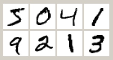
Let's try our softmax classifier on the MNIST handwritten digit classification dataset. Here are the first 8 images from MNIST, the goal is to look at the pixels and classify each image as one of the digits 0-9:
Load and minibatch the data. dtrn and dtst consist of xy pairs [ (x1,y1), (x2,y2), ... ] where xi,yi are minibatches of 100 instances:
using Knet
include(Knet.dir("data","mnist.jl"))
xtrn,ytrn,xtst,ytst = mnist()
dtst = minibatch(xtst,ytst,100)
dtrn = minibatch(xtrn,ytrn,100)
Here is the softmax classifier in Knet:
predict(w,x) = w[1]*mat(x) .+ w[2]	  # mat converts x to 2D
loss(w,x,ygold) = nll(predict(w,x),ygold) # nll computes negative log likelihood
lossgradient = grad(loss)                 # grad returns gradient function
wsoft=[ 0.1*randn(10,784), zeros(10,1) ]  # initial weights and bias
Here is the SGD training loop (see the full example in the Knet tutorial):
function train!(w, data; lr=.1)
    for (x,y) in data
        dw = lossgradient(w, x, y)
        for i in 1:length(w)
            w[i] -= lr * dw[i]
        end
    end
    return w
end
Here are the plots of the negative log likelihood and misclassification error vs training epochs:
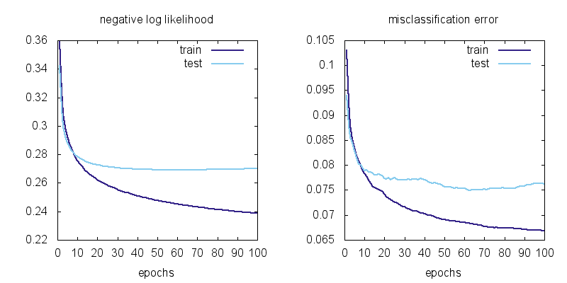
We can observe a few things. First the training losses are better than the test losses. This means there is some overfitting, i.e. the model is learning spurious regularities in the training data that do not generalize to test data. Second, it does not look like the training loss is going down to zero. This means there is also underfitting, i.e. the softmax model is not flexible enough to fit the training data exactly.
Representational power
So far we have seen how to create a machine learning model as a differentiable program (linear regression, softmax classification) whose parameters can be adjusted to hopefully imitate whatever process generated our training data. A natural question to ask is whether a particular model can behave like any system we want (given the right parameters) or whether there is a limit to what it can represent.
It turns out the softmax classifier is quite limited in its representational power: it can only represent linear classification boundaries. To show this, remember the form of the softmax classifier which gives the probability of the i'th class as:
\[p_i = \frac{\exp y_i}{\sum_{c=1}^C \exp y_c}\]
where $y_i$ is a linear function of the input $x$. Note that $p_i$ is a monotonically increasing function of $y_i$, so for two classes $i$ and $j$, $p_i > p_j$ iff $y_i > y_j$. The boundary between two classes $i$ and $j$ is the set of inputs for which the probability of the two classes are equal:
\[\begin{aligned} p_i &= p_j \\ y_i &= y_j \\ w_i x + b_i &= w_j x + b_j \\ (w_i - w_j) x + (b_i - b_j) &= 0 \end{aligned}\]
where $w_i, b_i$ refer to the i'th row of $w$ and $b$. This is a linear equation, i.e. the border between two classes will always be linear in the input space with the softmax classifier:
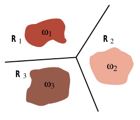
In the MNIST example, the relation between the pixels and the digit classes is unlikely to be this simple. That is why we are stuck at 6-7% training error. To get better results we need more powerful models.