Convolutional Neural Networks
Motivation
Let's say we are trying to build a model that will detect cats in photographs. The average resolution of images in ILSVRC is 482x415, with three channels (RGB) this makes the typical input size 482x415x3=600,090. Each hidden unit connected to the input in a multilayer perceptron would have 600K parameters, a single hidden layer of size 1000 would have 600 million parameters. Too many parameters cause three types of problems: (1) runtime: large models are computationally costly to train and run. (2) memory: today's GPUs have limited amount of memory (4G-12G) and large networks fill them up quickly. (3) sample complexity: models with a large number of parameters are difficult to train without overfitting: we need a lot of data, strong regularization, and/or a good initialization to learn with large models.
One problem with the MLP is that it is fully connected: every hidden unit is connected to every other in adjacent layers. The model does not assume any spatial relationships between pixels, in fact we can permute all the pixels in an image and the performance of the MLP would be the same! We could instead have an architecture where each hidden unit is connected to a small patch of the image, say 40x40. Each such locally connected hidden unit would have 40x40x3=4800 parameters instead of 600K. For the price (in memory) of one fully connected hidden unit (600K), we could have 125 of these locally connected mini-hidden-units (4800 each) with receptive fields spread around the image.
The second problem with the MLP is that it does not take advantage of the symmetry in the problem: a cat in the lower right corner of the image may be similar to a cat in the upper left corner. This means the local hidden units looking at these two patches can share the same weights. We can take one 40x40 cat filter and apply it to each 40x40 patch in the image taking up only 4800 parameters.
A convolutional neural network (aka CNN or ConvNet) combines these two ideas and uses operations that are local and that share weights. CNNs commonly use three types of operations: convolution, pooling, and normalization which we describe next.
Convolution
Convolution is the main operation that provides sparse connectivity and weight sharing. For simplicity we start describing convolution in 1-D using the conv4 primitive from Knet. We next look at three keyword options that provide variations on the convolution operation: padding, stride, and mode. We then describe how conv4 handles multiple dimensions, filters, and instances in parallel.
The relationship between convolution and matrix multiplication allows the use of efficient algorithms developed for matrix multiplication in convolution implementations. The fact that convolution and matrix multiplication can be implemented in terms of each other clarifies the distinction between CNNs and MLPs as one of efficiency, not representative power. We end this section by describing backpropagation for convolution.
Convolution in 1-D
Let $w, x$ be two 1-D vectors with $W, X$ elements respectively. In our examples, we will assume $x$ is the input (consider it a 1-D image) and $w$ is a filter (aka kernel) with $W<X$. The 1-D convolution operation $y=w\ast x$ results in a vector with $Y=X-W+1$ elements defined as:
\[y_k \equiv \sum_{i+j=k+W} x_i w_j\]
or equivalently
\[y_k \equiv \sum_{i=k}^{k+W-1} x_i w_{k+W-i}\]
where $i\in[1,X], j\in[1,W], k\in[1,Y]$. We get each entry in y by multiplying pairs of matching entries in x and w and summing the results. Matching entries in x and w are the ones whose indices add up to a constant. This can be visualized as flipping w, sliding it over x, and at each step writing their dot product into a single entry in y. Here is an example in Julia you should be able to calculate by hand:
julia> using Knet
julia> w = reshape([1.0,2.0,3.0], (3,1,1,1))
3×1×1×1 Array{Float64,4}: [1,2,3]
julia> x = reshape([1.0:7.0...], (7,1,1,1))
7×1×1×1 Array{Float64,4}: [1,2,3,4,5,6,7]
julia> y = conv4(w, x)
5×1×1×1 Array{Float64,4}: [10,16,22,28,34]
conv4 is the convolution operation in Knet (based on the CUDNN implementation). For reasons that will become clear it works with 4-D and 5-D arrays, so we reshape our 1-D input vectors by adding extra singleton dimensions at the end. The convolution of w=[1,2,3] and x=[1,2,3,4,5,6,7] gives y=[10,16,22,28,34]. For example, the third element of y, 22, can be obtained by reversing w to [3,2,1] and taking its dot product starting with the third element of x, [3,4,5].
Padding
In the last example, the input x had 7 dimensions, the output y had 5. In image processing applications we typically want to keep x and y the same size. For this purpose we can provide a padding keyword argument to the conv4 operator. If padding=k, x will be assumed padded with k zeros on the left and right before the convolution, e.g. padding=1 means treat x as [0 1 2 3 4 5 6 7 0]. The default padding is 0. For inputs in D-dimensions we can specify padding with a D-tuple, e.g. padding=(1,2) for 2D, or a single number, e.g. padding=1 which is shorthand for padding=(1,1). The result will have $Y=X+2P-W+1$ elements where $P$ is the padding size. Therefore to preserve the size of x when W=3 we should use padding=1.
julia> y = conv4(w, x; padding=(1,0))
7×1×1×1 Array{Float64,4}: [4,10,16,22,28,34,32]
For example, to calculate the first entry of y, take the dot product of the inverted w, [3,2,1] with the first three elements of the padded x, [0 1 2]. You can see that in order to preserve the input size, $Y=X$, given a filter size $W$, the padding should be set to $P=(W-1)/2$. This will work if $W$ is odd.
Stride
In the preceding examples we shift the inverted w by one position after each dot product. In some cases you may want to skip two or more positions. This will effectively reduce the size of the output. The amount of skip is set by the stride keyword argument of the conv4 operation (the default stride is 1). In the following example we set stride to $W$ such that the consecutive filter applications are non-overlapping:
julia> y = conv4(w, x; padding=(1,0), stride=3)
3×1×1×1 Array{Float64,4}: [4,22,32]
Note that the output has the first, middle, and last values of the previous example, i.e. every third value is kept and the rest are skipped. In general if stride=S and padding=P, the size of the output will be:
\[Y = 1 + \left\lfloor\frac{X+2P-W}{S}\right\rfloor\]
Mode
The convolution operation we have used so far flips the convolution kernel before multiplying it with the input. To take our first 1-D convolution example with
\[y_1 = x_1 w_W + x_2 w_{W-1} + x_3 w_{W-2} + \ldots \\ y_2 = x_2 w_W + x_3 w_{W-1} + x_4 w_{W-2} + \ldots \\ \ldots\]
We could also perform a similar operation without kernel flipping:
\[y_1 = x_1 w_1 + x_2 w_2 + x_3 w_3 + \ldots \\ y_2 = x_2 w_1 + x_3 w_2 + x_4 w_3 + \ldots \\ \ldots\]
This variation is called cross-correlation. The two modes are specified in Knet by choosing one of the following as the value of the mode keyword:
0for convolution1for cross-correlation
This option would be important if we were hand designing our filters. However the mode does not matter for CNNs where the filters are learnt from data, the CNN will simply learn an inverted version of the filter if necessary.
More Dimensions
When the input x has multiple dimensions convolution is defined similarly. In particular the filter w has the same number of dimensions but typically smaller size. The convolution operation flips w in each dimension and slides it over x, calculating the sum of elementwise products at every step. The formulas we have given above relating the output size to the input and filter sizes, padding and stride parameters apply independently for each dimension.
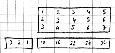
Knet supports 2D and 3D convolutions. The inputs and the filters have two extra dimensions at the end which means we use 4D and 5D arrays for 2D and 3D convolutions. Here is a 2D convolution example:
julia> w = reshape([1.0:4.0...], (2,2,1,1))
2×2×1×1 Array{Float64,4}:
[:, :, 1, 1] =
 1.0  3.0
 2.0  4.0
julia> x = reshape([1.0:9.0...], (3,3,1,1))
3×3×1×1 Array{Float64,4}:
[:, :, 1, 1] =
 1.0  4.0  7.0
 2.0  5.0  8.0
 3.0  6.0  9.0
julia> y = conv4(w, x)
2×2×1×1 Array{Float64,4}:
[:, :, 1, 1] =
 23.0  53.0
 33.0  63.0
To see how this result comes about, note that when you flip w in both dimensions you get:
4 2
3 1
Multiplying this elementwise with the upper left corner of x:
1 4
2 5
and adding the results gives you the first entry 23.
The padding and stride options work similarly in multiple dimensions and can be specified as tuples: padding=(1,2) means a padding width of 1 along the first dimension and 2 along the second dimension for a 2D convolution. You can use padding=1 as a shorthand for padding=(1,1).
Multiple filters
So far we have been ignoring the extra dimensions at the end of our convolution arrays. Now we are ready to put them to use. A D-dimensional input image is typically represented as a D+1 dimensional array with dimensions:
\[[ X_1, \ldots, X_D, C_x ]\]
The first D dimensions $X_1\ldots X_D$ determine the spatial extent of the image. The last dimension $C_x$ is the number of channels (aka slices, frames, maps, filters). The definition and number of channels is application dependent. We use $C_x=3$ for RGB images representing the intensity in three colors: red, green, and blue. For grayscale images we have a single channel, $C_x=1$. If you were developing a model for chess, we could have $C_x=12$, each channel representing the locations of a different piece type.
In an actual CNN we do not typically hand-code the filters. Instead we tell the network: "here are 1000 randomly initialized filters, you go ahead and turn them into patterns useful for my task." This means we usually work with banks of multiple filters simultaneously and GPUs have optimized operations for such filter banks. The dimensions of a typical filter bank are:
\[[ W_1, \ldots, W_D, C_x, C_y ]\]
The first D dimensions $W_1\ldots W_D$ determine the spatial extent of the filters. The next dimension $C_x$ is the number of input channels, i.e. the number of filters from the previous layer, or the number of color channels of the input image. The last dimension $C_y$ is the number of output channels, i.e. the number of filters in this layer.
If we take an input of size $[X_1,\ldots, X_D,C_x]$ and apply a filter bank of size $[W_1,\ldots,W_D,C_x,C_y]$ using padding $[P_1,\ldots,P_D]$ and stride $[S_1,\ldots,S_D]$ the resulting array will have dimensions:
\[[ W_1, \ldots, W_D, C_x, C_y ] \ast [ X_1, \ldots, X_D, C_x ] \Rightarrow [ Y_1, \ldots, Y_D, C_y ] \\ \mathrm{where } Y_i = 1 + \left\lfloor\frac{X_i+2P_i-W_i}{S_i}\right\rfloor\]
As an example let's start with an input image of 256x256 pixels and 3 RGB channels. We'll first apply 25 filters of size 5x5 and padding=2, then 50 filters of size 3x3 and padding=1, and finally 75 filters of size 3x3 and padding=1. Here are the dimensions we will get:
\[[ 256, 256, 3 ] \ast [ 5, 5, 3, 25 ] \Rightarrow [ 256, 256, 25 ] \\ [ 256, 256, 25] \ast [ 3, 3, 25,50 ] \Rightarrow [ 256, 256, 50 ] \\ [ 256, 256, 50] \ast [ 3, 3, 50,75 ] \Rightarrow [ 256, 256, 75 ]\]
Note that the number of input channels of the input data and the filter bank always match. In other words, a filter covers only a small part of the spatial extent of the input but all of its channel depth.
Multiple instances
In addition to processing multiple filters in parallel, we implement CNNs with minibatching, i.e. process multiple inputs in parallel to fully utilize GPUs. A minibatch of D-dimensional images is represented as a D+2 dimensional array:
\[[ X_1, \ldots, X_D, C_x, N ]\]
where $C_x$ is the number of channels as before, and N is the number of images in a minibatch. The convolution implementation in Knet/CUDNN use $D+2$ dimensional arrays for both images and filters. We used 1 for the extra dimensions in our first examples, in effect using a single channel and a single image minibatch.
If we apply a filter bank of size $[W_1, \ldots, W_D, C_x, C_y]$ to the minibatch given above the output size would be:
\[[ W_1, \ldots, W_D, C_x, C_y ] \ast [ X_1, \ldots, X_D, C_x, N ] \Rightarrow [ Y_1, \ldots, Y_D, C_y, N ] \\ \mathrm{where } Y_i = 1 + \left\lfloor\frac{X_i+2P_i-W_i}{S_i}\right\rfloor\]
If we used a minibatch size of 128 in the previous example with 256x256 images, the sizes would be:
\[[ 256, 256, 3, 128 ] \ast [ 5, 5, 3, 25 ] \Rightarrow [ 256, 256, 25, 128 ] \\ [ 256, 256, 25, 128] \ast [ 3, 3, 25,50 ] \Rightarrow [ 256, 256, 50, 128 ] \\ [ 256, 256, 50, 128] \ast [ 3, 3, 50,75 ] \Rightarrow [ 256, 256, 75, 128 ]\]
basically adding an extra dimension of 128 at the end of each data array.
By the way, the arrays in this particular example already exceed 5GB of storage, so you would want to use a smaller minibatch size if you had a K20 GPU with 4GB of RAM.
Note: All the dimensions given above are for column-major languages like Julia. CUDNN uses row-major notation, so all the dimensions would be reversed, e.g. $[N,C_x,X_D,\ldots,X_1]$.
Convolution vs matrix multiplication
Convolution can be turned into a matrix multiplication, where certain entries in the matrix are constrained to be the same. The motivation is to be able to use efficient algorithms for matrix multiplication in order to perform convolution. The drawback is the large amount of memory needed due to repeated entries or sparse representations.
Here is a matrix implementation for our first convolution example $w=[1\ldots 3],\,\,x=[1\ldots 7],\,\,w\ast x = [10,16,22,28,34]$:
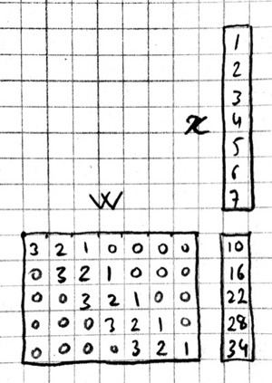
In this example we repeated the entries of the filter on multiple rows of a sparse matrix with shifted positions. Alternatively we can repeat the entries of the input to place each local patch on a separate column of an input matrix:
The first approach turns w into a $Y\times X$ sparse matrix, wheras the second turns x into a $W\times Y$ dense matrix.
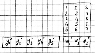
For 2-D images, typically the second approach is used: the local patches of the image used by convolution are stretched out to columns of an input matrix, an operation commonly called im2col. Each convolutional filter is stretched out to rows of a filter matrix. After the matrix multiplication the resulting array is reshaped into the proper output dimensions. The following figure illustrates these operations on a small example:
It is also possible to go in the other direction, i.e. implement matrix multiplication (i.e. a fully connected layer) in terms of convolution. This conversion is useful when we want to build a network that can be applied to inputs of different sizes: the matrix multiplication would fail, but the convolution will give us outputs of matching sizes. Consider a fully connected layer with a weight matrix W of size $K\times D$ mapping a D-dimensional input vector x to a K-dimensional output vector y. We can consider each of the K rows of the W matrix a convolution filter. The following example shows how we can reshape the arrays and use convolution for matrix multiplication:
julia> using Knet
julia> x = reshape([1.0:3.0...], (3,1))
3×1 Array{Float64,2}:
 1.0
 2.0
 3.0
julia> w = reshape([1.0:6.0...], (2,3))
2×3 Array{Float64,2}:
 1.0  3.0  5.0
 2.0  4.0  6.0
julia> y = w * x
2×1 Array{Float64,2}:
 22.0
 28.0
julia> x2 = reshape(x, (3,1,1,1))
3×1×1×1 Array{Float64,4}:
[:, :, 1, 1] =
 1.0
 2.0
 3.0
julia> w2 = reshape(Array(w)', (3,1,1,2))
3×1×1×2 Array{Float64,4}:
[:, :, 1, 1] =
 1.0
 3.0
 5.0
[:, :, 1, 2] =
 2.0
 4.0
 6.0
julia> y2 = conv4(w2, x2; mode=1)
1×1×2×1 Array{Float64,4}:
[:, :, 1, 1] =
 22.0
[:, :, 2, 1] =
 28.0
In addition to computational concerns, these examples also show that a fully connected layer can emulate a convolutional layer given the right weights and vice versa, i.e. convolution does not get us any extra representational power. However it does get us representational and statistical efficiency, i.e. the functions we would like to approximate are often expressed with significantly fewer parameters using convolutional layers and thus require fewer examples to train.
Backpropagation
Convolution is a linear operation consisting of additions and multiplications, so its backward pass is not very complicated except for the indexing. Just like the backward pass for matrix multiplication can be expressed as another matrix multiplication, the backward pass for convolution (at least if we use stride=1) can be expressed as another convolution. We will derive the backward pass for a 1-D example using the cross-correlation mode (no kernel flipping) to keep things simple. We will denote the cross-correlation operation with $\star$ to distinguish it from convolution denoted with $\ast$. Here are the individual entries of $y=w\star x$:
\[y_1 = x_1 w_1 + x_2 w_2 + x_3 w_3 + \ldots \\ y_2 = x_2 w_1 + x_3 w_2 + x_4 w_3 + \ldots \\ y_3 = x_3 w_1 + x_4 w_2 + x_5 w_3 + \ldots \\ \ldots\]
As you can see, because of weight sharing the same w entry is used in computing multiple y entries. This means a single w entry effects the objective function through multiple paths and these effects need to be added. Denoting $\partial J/\partial y_i$ as $y_i'$ for brevity we have:
\[w_1' = x_1 y_1' + x_2 y_2' + \ldots \\ w_2' = x_2 y_1' + x_3 y_2' + \ldots \\ w_3' = x_3 y_1' + x_4 y_2' + \ldots \\ \ldots \\\]
which can be recognized as another cross-correlation operation, this time between $x$ and $y'$. This allows us to write $w'=y'\star x$.
Alternatively, we can use the equivalent matrix multiplication operation from the last section to derive the backward pass:
If $r$ is the matrix with repeated $x$ entries in this picture, we have $y=wr$. Remember that the backward pass for matrix multiplication $y=wr$ is $w'=y'r^T$:
which can be recognized as the matrix multiplication equivalent of the cross correlation operation $w'=y'\star x$.
Here is the gradient for the input:
\[\begin{aligned} & x_1' = w_1 y_1' \\ & x_2' = w_2 y_1' + w_1 y_2' \\ & x_3' = w_3 y_1' + w_2 y_2' + w_1 y_3' \\ & \ldots \end{aligned}\]
You can recognize this as a regular convolution between $w$ and $y'$ with some zero padding.
The following resources provide more detailed derivations of the backward pass for convolution:
- Goodfellow, I. (2010). Technical report: Multidimensional, downsampled convolution for autoencoders. Technical report, Université de Montréal. 312.
- Bouvrie, J. (2006). Notes on convolutional neural networks.
- UFLDL tutorial and exercise on CNNs.
Pooling
It is common practice to use pooling (aka subsampling) layers in between convolution operations in CNNs. Pooling looks at small windows of the input, and computes a single summary statistic, e.g. maximum or average, for each window. A pooling layer basically says: tell me whether this feature exists in a certain region of the image, I don't care exactly where. This makes the output of the layer invariant to small translations of the input. Pooling layers use large strides, typically as large as the window size, which reduces the size of their output.
Like convolution, pooling slides a small window of a given size over the input optionally padded with zeros skipping stride pixels every step. In Knet by default there is no padding, the window size is 2, stride is equal to the window size and the pooling operation is max. These default settings reduce each dimension of the input to half the size.
Pooling in 1-D
Here is a 1-D example:
julia> x = reshape([1.0:6.0...], (6,1,1,1))
6×1×1×1 Array{Float64,4}: [1,2,3,4,5,6]
julia> pool(x)
3×1×1×1 Array{Float64,4}: [2,4,6]
With window size and stride equal to 2, pooling considers the input windows $[1,2], [3,4], [5,6]$ and picks the maximum in each window.
Window
The default and most commonly used window size is 2, however other window sizes can be specified using the window keyword. For D-dimensional inputs the size can be specified using a D-tuple, e.g. window=(2,3) for 2-D, or a single number, e.g. window=3 which is shorthand for window=(3,3) in 2-D. Here is an example using a window size of 3 instead of the default 2:
julia> x = reshape([1.0:6.0...], (6,1,1,1))
6×1×1×1 Array{Float64,4}: [1,2,3,4,5,6]
julia> pool(x; window=3)
2×1×1×1 Array{Float64,4}: [3, 6]
With a window and stride of 3 (the stride is equal to window size by default), pooling considers the input windows $[1,2,3],[4,5,6]$, and writes the maximum of each window to the output. If the input size is $X$, and stride is equal to the window size $W$, the output will have $Y=\lfloor X/W\rfloor$ elements.
Padding
The amount of zero padding is specified using the padding keyword argument just like convolution. Padding is 0 by default. For D-dimensional inputs padding can be specified as a tuple such as padding=(1,2), or a single number padding=1 which is shorthand for padding=(1,1) in 2-D. Here is a 1-D example:
julia> x = reshape([1.0:6.0...], (6,1,1,1))
6×1×1×1 Array{Float64,4}: [1,2,3,4,5,6]

julia> pool(x; padding=(1,0))
4×1×1×1 Array{Float64,4}: [1,3,5,6]
In this example, window=stride=2 by default and the padding size is 1, so the input is treated as $[0,1,2,3,4,5,6,0]$ and split into windows of $[0,1],[2,3],[4,5],[6,0]$ and the maximum of each window is written to the output.
With padding size $P$, if the input size is $X$, and stride is equal to the window size $W$, the output will have $Y=\lfloor (X+2P)/W\rfloor$ elements.
Stride
The pooling stride is equal to the window size by default (as opposed to the convolution case, where it is 1 by default). This is most common in practice but other strides can be specified using tuples e.g. stride=(1,2) or numbers e.g. stride=1. Here is a 1-D example with a stride of 4 instead of the default 2:
julia> x = reshape([1.0:10.0...], (10,1,1,1))
10×1×1×1 Array{Float64,4}: [1,2,3,4,5,6,7,8,9,10]

julia> pool(x; stride=4)
4×1×1×1 Array{Float64,4}: [2, 6, 10]
In general, when we have an input of size $X$ and pool with window size $W$, padding $P$, and stride $S$, the size of the output will be:
\[Y = 1 + \left\lfloor\frac{X+2P-W}{S}\right\rfloor\]
Mode
There are three pooling operations defined by CUDNN used for summarizing each window:
CUDNN_POOLING_MAXCUDNN_POOLING_AVERAGE_COUNT_INCLUDE_PADDINGCUDNN_POOLING_AVERAGE_COUNT_EXCLUDE_PADDING
These options can be specified as the value of the mode keyword argument to the pool operation. The default is 0 (max pooling) which we have been using so far. The last two compute averages, and differ in whether to include or exclude the padding zeros in these averages. mode should be 1 for averaging including padding, and 2 for averaging excluding padding. For example, with input $x=[1,2,3,4,5,6]$, window=stride=2, and padding=1 we have the following outputs with the three options:
mode=0 => [1,3,5,6]
mode=1 => [0.5, 2.5, 4.5, 3.0]
mode=2 => [1.0, 2.5, 4.5, 6.0]
More Dimensions
D-dimensional inputs are pooled with D-dimensional windows, the size of each output dimension given by the 1-D formulas above. Here is a 2-D example with default options, i.e. window=stride=(2,2), padding=(0,0), mode=max:
julia> x = reshape([1.0:16.0...], (4,4,1,1))
4×4×1×1 Array{Float64,4}:
[:, :, 1, 1] =
 1.0  5.0   9.0  13.0
 2.0  6.0  10.0  14.0
 3.0  7.0  11.0  15.0
 4.0  8.0  12.0  16.0

julia> pool(x)
2×2×1×1 Array{Float64,4}:
[:, :, 1, 1] =
 6.0  14.0
 8.0  16.0
Multiple channels and instances
As we saw in convolution, each data array has two extra dimensions in addition to the spatial dimensions: $[ X_1, \ldots, X_D, C_x, N ]$ where $C_x$ is the number of channels and $N$ is the number of instances in a minibatch.
When the number of channels is greater than 1, the pooling operation is performed independently on each channel, e.g. for each patch, the maximum/average in each channel is computed independently and copied to the output. Here is an example with two channels:
julia> x = rand(4,4,2,1)
4×4×2×1 Array{Float64,4}:
[:, :, 1, 1] =
 0.880221  0.738729  0.317231   0.990521
 0.626842  0.562692  0.339969   0.92469
 0.416676  0.403625  0.352799   0.46624
 0.566254  0.634703  0.0632812  0.0857779

[:, :, 2, 1] =
 0.300799  0.407623   0.26275   0.767884
 0.217025  0.0055375  0.623168  0.957374
 0.154975  0.246693   0.769524  0.628197
 0.259161  0.648074   0.333324  0.46305

julia> pool(x)
2×2×2×1 Array{Float64,4}:
[:, :, 1, 1] =
 0.880221  0.990521
 0.634703  0.46624

[:, :, 2, 1] =
 0.407623  0.957374
 0.648074  0.769524
When the number of instances is greater than 1, i.e. we are using minibatches, the pooling operation similarly runs in parallel on all the instances:
julia> x = rand(4,4,1,2)
4×4×1×2 Array{Float64,4}:
[:, :, 1, 1] =
 0.155228  0.848345  0.629651  0.262436
 0.729994  0.320431  0.466628  0.0293943
 0.374592  0.662795  0.819015  0.974298
 0.421283  0.83866   0.385306  0.36081

[:, :, 1, 2] =
 0.0562608  0.598084  0.0231604  0.232413
 0.71073    0.411324  0.28688    0.287947
 0.997445   0.618981  0.471971   0.684064
 0.902232   0.570232  0.190876   0.339076

julia> pool(x)
2×2×1×2 Array{Float64,4}:
[:, :, 1, 1] =
 0.848345  0.629651
 0.83866   0.974298

[:, :, 1, 2] =
 0.71073   0.287947
 0.997445  0.684064
Normalization
Draft...
Karpathy says: "Many types of normalization layers have been proposed for use in ConvNet architectures, sometimes with the intentions of implementing inhibition schemes observed in the biological brain. However, these layers have recently fallen out of favor because in practice their contribution has been shown to be minimal, if any." (http://cs231n.github.io/convolutional-networks/#norm) Batch normalization may be an exception, as it is used in modern architectures.
Here are some references for normalization operations:
Implementations:
- Alex Krizhevsky's cuda-convnet library API. (https://code.google.com/archive/p/cuda-convnet/wikis/LayerParams.wiki#Localresponsenormalizationlayer(same_map))
- http://caffe.berkeleyvision.org/tutorial/layers.html
- http://lasagne.readthedocs.org/en/latest/modules/layers/normalization.html
Divisive normalisation (DivN):
- S. Lyu and E. Simoncelli. Nonlinear image representation using divisive normalization. In CVPR, pages 1–8, 2008.
Local contrast normalization (LCN):
- N. Pinto, D. D. Cox, and J. J. DiCarlo. Why is real-world visual object recognition hard? PLoS Computational Biology, 4(1), 2008.
- Jarrett, Kevin, et al. "What is the best multi-stage architecture for object recognition?." Computer Vision, 2009 IEEE 12th International Conference on. IEEE, 2009. (http://yann.lecun.com/exdb/publis/pdf/jarrett-iccv-09.pdf)
Local response normalization (LRN):
- Krizhevsky, Alex, Ilya Sutskever, and Geoffrey E. Hinton. "Imagenet classification with deep convolutional neural networks." Advances in neural information processing systems. 2012. (http://machinelearning.wustl.edu/mlpapers/paperfiles/NIPS20120534.pdf)
Batch Normalization: This is more of an optimization topic.
- Ioffe, Sergey, and Christian Szegedy. "Batch normalization: Accelerating deep network training by reducing internal covariate shift." arXiv preprint arXiv:1502.03167 (2015). (http://arxiv.org/abs/1502.03167/)
Architectures
We have seen a number of new operations: convolution, pooling, filters etc. How to best put these together to form a CNN is still an active area of research. In this section we summarize common patterns of usage in recent work based on (Karpathy, 2016).
- The operations in convolutional networks are usually ordered into several layers of convolution-bias-activation-pooling sequences. Note that the convolution-bias-activation sequence is an efficient way to implement the common neural net function $f(wx+b)$ for a locally connected and weight sharing hidden layer.
- The convolutional layers are typically followed by a number of fully connected layers that end with a softmax layer for prediction (if we are training for a classification problem).
- It is preferrable to have multiple convolution layers with small filter sizes rather than a single layer with a large filter size. Consider three convolutional layers with a filter size of 3x3. The units in the top layer have receptive fields of size 7x7. Compare this with a single layer with a filter size of 7x7. The three layer architecture has two advantages: The units in the single layer network is restricted to linear decision boundaries, whereas the three layer network can be more expressive. Second, if we assume C channels, the parameter tensor for the single layer network has size $[7,7,C,C]$ whereas the three layer network has three tensors of size $[3,3,C,C]$ i.e. a smaller number of parameters. The one disadvantage of the three layer network is the extra storage required to store the intermediate results for backpropagation.
- Thus common settings for convolution use 3x3 filters with
stride = padding = 1(which incidentally preserves the input size). The one exception may be a larger filter size used in the first layer which is applied to the image pixels. This will save memory when the input is at its largest, and linear functions may be sufficient to express the low level features at this stage. - The pooling operation may not be present in every layer. Keep in mind that pooling destroys information and having several convolutional layers without pooling may allow more complex features to be learnt. When pooling is present it is best to keep the window size small to minimize information loss. The common settings for pooling are
window = stride = 2, padding = 0, which halves the input size in each dimension.
Beyond these general guidelines, you should look at the architectures used by successful models in the literature. Some examples are LeNet (LeCun et al. 1998), AlexNet (Krizhevsky et al. 2012), ZFNet (Zeiler and Fergus, 2013), GoogLeNet (Szegedy et al. 2014), VGGNet (Simonyan and Zisserman, 2014), and ResNet (He et al. 2015).
Exercises
- Design a filter that shifts a given image one pixel to right.
- Design an image filter that has 0 output in regions of uniform color, but nonzero output at edges where the color changes.
- If your input consisted of two consecutive frames of video, how would you detect motion using convolution?
- Can you implement matrix-vector multiplication in terms of convolution? How about matrix-matrix multiplication? Do you need reshape operations?
- Can you implement convolution in terms of matrix multiplication?
- Can you implement elementwise broadcasting multiplication in terms of convolution?
References
- Some of this chapter was based on the excellent lecture notes from: http://cs231n.github.io/convolutional-networks
- Christopher Olah's blog has very good visual explanations (thanks to Melike Softa for the reference): http://colah.github.io/posts/2014-07-Conv-Nets-Modular
- http://yosinski.com/deepvis
- https://distill.pub/2017/feature-visualization/
- https://distill.pub/2018/building-blocks/
- UFLDL (or its old version) is an online tutorial with programming examples and explicit gradient derivations covering convolution, pooling, and CNNs.
- Hinton's video lecture and presentation at Coursera (Lec 5): https://d396qusza40orc.cloudfront.net/neuralnets/lecture_slides/lec5.pdf
- For a derivation of gradients see: http://people.csail.mit.edu/jvb/papers/cnn_tutorial.pdf or http://www.iro.umontreal.ca/~lisa/pointeurs/convolution.pdf
- The CUDNN manual has more details about the convolution API: https://developer.nvidia.com/cudnn
- http://deeplearning.net/tutorial/lenet.html
- http://www.denizyuret.com/2014/04/on-emergence-of-visual-cortex-receptive.html
- http://neuralnetworksanddeeplearning.com/chap6.html
- http://www.deeplearningbook.org/contents/convnets.html
- http://www.wildml.com/2015/11/understanding-convolutional-neural-networks-for-nlp
- http://scs.ryerson.ca/~aharley/vis/conv/ has a nice visualization of an MNIST CNN. (Thanks to Fatih Ozhamaratli for the reference).
- http://josephpcohen.com/w/visualizing-cnn-architectures-side-by-side-with-mxnet visualizing popular CNN architectures side by side with mxnet.
- http://cs231n.github.io/understanding-cnn visualizing what convnets learn.
- https://arxiv.org/abs/1603.07285 A guide to convolution arithmetic for deep learning
- Reading (architectures): cs231n Architecture Slides
- Reading (visualization): cs231n Visualization Slides, cs231n Visualization Notes, Distillpub visualization article, Yosinski blog, video, paper, repo
- A Simple Guide to the Versions of the Inception Network