Introduction to Knet
![]()


Knet (pronounced "kay-net") is the Koç University deep learning framework implemented in Julia by Deniz Yuret and collaborators. It supports GPU operation and automatic differentiation using dynamic computational graphs for models defined in plain Julia. This document is a tutorial introduction to Knet. Check out the full documentation and Examples for more information. If you need help or would like to request a feature, please consider joining the knet-users mailing list. If you find a bug, please open a GitHub issue. If you would like to contribute to Knet development, check out the knet-dev mailing list and Tips for developers. If you use Knet in academic work, here is a paper that can be cited:
@inproceedings{knet2016mlsys,
  author={Yuret, Deniz},
  title={Knet: beginning deep learning with 100 lines of Julia},
  year={2016},
  booktitle={Machine Learning Systems Workshop at NIPS 2016}
}
Contents
Philosophy
Knet uses dynamic computational graphs generated at runtime for automatic differentiation of (almost) any Julia code. This allows machine learning models to be implemented by defining just the forward calculation (i.e. the computation from parameters and data to loss) using the full power and expressivity of Julia. The implementation can use helper functions, loops, conditionals, recursion, closures, tuples and dictionaries, array indexing, concatenation and other high level language features, some of which are often missing in the restricted modeling languages of static computational graph systems like Theano, Torch, Caffe and Tensorflow. GPU operation is supported by simply using the KnetArray type instead of regular Array for parameters and data.
Knet builds a dynamic computational graph by recording primitive operations during forward calculation. Only pointers to inputs and outputs are recorded for efficiency. Therefore array overwriting is not supported during forward and backward passes. This encourages a clean functional programming style. High performance is achieved using custom memory management and efficient GPU kernels. See Under the hood for more details.
Tutorial
In Knet, a machine learning model is defined using plain Julia code. A typical model consists of a prediction and a loss function. The prediction function takes model parameters and some input, returns the prediction of the model for that input. The loss function measures how bad the prediction is with respect to some desired output. We train a model by adjusting its parameters to reduce the loss. In this section we will see the prediction, loss, and training functions for five models: linear regression, softmax classification, fully-connected, convolutional and recurrent neural networks. It would be best to copy paste and modify these examples on your own computer. They are also available as an IJulia notebook. You can install Knet using Pkg.add("Knet") in Julia.
Linear regression
Here is the prediction function and the corresponding quadratic loss function for a simple linear regression model:
using Knet

predict(w,x) = w[1]*x .+ w[2]

loss(w,x,y) = mean(abs2,y-predict(w,x))
The variable w is a list of parameters (it could be a Tuple, Array, or Dict), x is the input and y is the desired output. To train this model, we want to adjust its parameters to reduce the loss on given training examples. The direction in the parameter space in which the loss reduction is maximum is given by the negative gradient of the loss. Knet uses the higher-order function grad from AutoGrad.jl to compute the gradient direction:
lossgradient = grad(loss)Note that grad is a higher-order function that takes and returns other functions. The lossgradient function takes the same arguments as loss, e.g. dw = lossgradient(w,x,y). Instead of returning a loss value, lossgradient returns dw, the gradient of the loss with respect to its first argument w. The type and size of dw is identical to w, each entry in dw gives the derivative of the loss with respect to the corresponding entry in w.
Given some training data = [(x1,y1),(x2,y2),...], here is how we can train this model:
function train(w, data; lr=.1)
    for (x,y) in data
        dw = lossgradient(w, x, y)
	for i in 1:length(w)
	    w[i] -= lr * dw[i]
	end
    end
    return w
end
We simply iterate over the input-output pairs in data, calculate the lossgradient for each example, and move the parameters in the negative gradient direction with a step size determined by the learning rate lr.

Let's train this model on the Boston Housing dataset from the UCI Machine Learning Repository.
include(Knet.dir("data","housing.jl"))
x,y = housing()
w = Any[ 0.1*randn(1,13), 0.0 ]
for i=1:10; train(w, [(x,y)]); println(loss(w,x,y)); end
# 366.0463078055053
# ...
# 29.63709385230451
The dataset has housing related information for 506 neighborhoods in Boston from 1978. Each neighborhood is represented using 13 attributes such as crime rate or distance to employment centers. The goal is to predict the median value of the houses given in $1000's. The housing() function from housing.jl downloads, splits and normalizes the data. We initialize the parameters randomly and take 10 steps in the negative gradient direction. We can see the loss dropping from 366.0 to 29.6. See the housing example for more information on this model.
Note that grad was the only function used that is not in the Julia standard library. This is typical of models defined in Knet, where most of the code is written in plain Julia.
Softmax classification
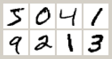
In this example we build a simple classification model for the MNIST handwritten digit recognition dataset. MNIST has 60000 training and 10000 test examples. Each input x consists of 784 pixels representing a 28x28 image. The corresponding output indicates the identity of the digit 0..9.
Classification models handle discrete outputs, as opposed to regression models which handle numeric outputs. We typically use the cross entropy loss function in classification models:
predict(w,x) = w[1]*mat(x) .+ w[2]

loss(w,x,ygold) = nll(predict(w,x), ygold)

lossgradient = grad(loss)
nll computes the negative log likelihood of your predictions compared to the correct answers. Here, we assume ygold is an array of N integers indicating the correct answers for N instances (we use ygold=10 to represent the 0 answer) and predict() gives us a (10,N) matrix of scores for each answer. mat is needed to convert the (28,28,1,N) x array to a (784,N) matrix so it can be used in matrix multiplication. Other than the change of loss function, the softmax model is identical to the linear regression model. We use the same predict (except for mat reshaping), train and set lossgradient=grad(loss) as before.
Now let's train a model on the MNIST data:
include(Knet.dir("data","mnist.jl"))
xtrn, ytrn, xtst, ytst = mnist()
dtrn = minibatch(xtrn, ytrn, 100)
dtst = minibatch(xtst, ytst, 100)
w = Any[ 0.1f0*randn(Float32,10,784), zeros(Float32,10,1) ]
println((:epoch, 0, :trn, accuracy(w,dtrn,predict), :tst, accuracy(w,dtst,predict)))
for epoch=1:10
    train(w, dtrn; lr=0.5)
    println((:epoch, epoch, :trn, accuracy(w,dtrn,predict), :tst, accuracy(w,dtst,predict)))
end

# (:epoch,0,:trn,0.11761667f0,:tst,0.121f0)
# (:epoch,1,:trn,0.9005f0,:tst,0.9048f0)
# ...
# (:epoch,10,:trn,0.9196f0,:tst,0.9153f0)
Calling mnist() from mnist.jl loads the MNIST data, downloading it from the internet if necessary, and provides a training set (xtrn,ytrn) and a test set (xtst,ytst). minibatch is used to rearrange the data into chunks of 100 instances. After randomly initializing the parameters we train for 10 epochs, printing out training and test set accuracy at every epoch. The final accuracy of about 92% is close to the limit of what we can achieve with this type of model. To improve further we must look beyond linear models.
Multi-layer perceptron
A multi-layer perceptron, i.e. a fully connected feed-forward neural network, is basically a bunch of linear regression models stuck together with non-linearities in between.
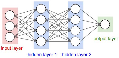
We can define a MLP by slightly modifying the predict function:
function predict(w,x)
    x = mat(x)
    for i=1:2:length(w)-2
        x = relu.(w[i]*x .+ w[i+1])
    end
    return w[end-1]*x .+ w[end]
end
Here w[2k-1] is the weight matrix and w[2k] is the bias vector for the k'th layer. relu implements the popular rectifier non-linearity: relu.(x) = max.(0,x). Note that if w only has two entries, this is equivalent to the linear and softmax models. By adding more entries to w, we can define multi-layer perceptrons of arbitrary depth. Let's define one with a single hidden layer of 64 units:
w = Any[ 0.1f0*randn(Float32,64,784), zeros(Float32,64,1),
         0.1f0*randn(Float32,10,64),  zeros(Float32,10,1) ]
The rest of the code is the same as the softmax model. We can use the same cross-entropy loss function and the same training script. However, we will use a different train function to introduce alternative optimizers:
function train(model, data, optim)
    for (x,y) in data
        grads = lossgradient(model,x,y)
        update!(model, grads, optim)
    end
end
Here the optim argument specifies the optimization algorithm and state for each model parameter (see Optimization methods for available algorithms). update! uses optim to update each model parameter and optimization state. optim has the same size and shape as model, i.e. we have a separate optimizer for each model parameter. For simplicity we will use the optimizers function to create an Adam optimizer for each parameter:
o = optimizers(w, Adam)
println((:epoch, 0, :trn, accuracy(w,dtrn,predict), :tst, accuracy(w,dtst,predict)))
for epoch=1:10
    train(w, dtrn, o)
    println((:epoch, epoch, :trn, accuracy(w,dtrn,predict), :tst, accuracy(w,dtst,predict)))
end
The code for this example is available in the mnist-mlp example or the knet-tutorial notebook. The multi-layer perceptron does significantly better than the softmax model:
(:epoch,0,:trn,0.10166667f0,:tst,0.0977f0)
(:epoch,1,:trn,0.9389167f0,:tst,0.9407f0)
...
(:epoch,10,:trn,0.9866f0,:tst,0.9735f0)
Convolutional neural network
To improve the performance further, we can use a convolutional neural networks (CNN). See the course notes by Andrej Karpathy for a good introduction to CNNs. We will implement the LeNet model which consists of two convolutional layers followed by two fully connected layers.
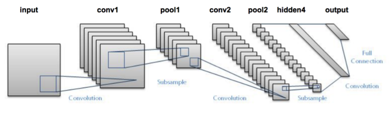
Knet provides the conv4 and pool functions for the implementation of convolutional nets:
function predict(w,x0)
    x1 = pool(relu.(conv4(w[1],x0) .+ w[2]))
    x2 = pool(relu.(conv4(w[3],x1) .+ w[4]))
    x3 = relu.(w[5]*mat(x2) .+ w[6])
    return w[7]*x3 .+ w[8]
end
The weights for the convolutional net can be initialized as follows.
w = Any[ xavier(Float32,5,5,1,20),  zeros(Float32,1,1,20,1),
         xavier(Float32,5,5,20,50), zeros(Float32,1,1,50,1),
         xavier(Float32,500,800),   zeros(Float32,500,1),
         xavier(Float32,10,500),    zeros(Float32,10,1) ]
Here we used xavier instead of randn which initializes weights based on their input and output widths.
This model is larger and more expensive to train compared to the previous models we have seen and it would be nice to use our GPU. To perform the operations on the GPU, all we need to do is to convert our data and weights to KnetArrays. minibatch takes an extra keyword argument xtype for this purpose, and we do it manually for the w weights:
dtrn = minibatch(xtrn,ytrn,100,xtype=KnetArray)
dtst = minibatch(xtst,ytst,100,xtype=KnetArray)
w = map(KnetArray, w)
The training proceeds as before giving us even better results. The code for the LeNet example can be found under the examples directory.
(:epoch, 0, :trn, 0.10435, :tst, 0.103)
(:epoch, 1, :trn, 0.98385, :tst, 0.9836)
...
(:epoch, 10, :trn, 0.9955166666666667, :tst, 0.9902)
Recurrent neural network
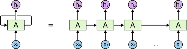
In this section we will see how to implement a recurrent neural network (RNN) in Knet. This example, like the last one, requires a GPU. An RNN is a class of neural network where connections between units form a directed cycle, which allows them to keep a persistent state over time. This gives them the ability to process sequences of arbitrary length one element at a time, while keeping track of what happened at previous elements.
As an example, we will build a character-level language model inspired by "The Unreasonable Effectiveness of Recurrent Neural Networks" from the Andrej Karpathy blog. The model can be trained with different genres of text, and can be used to generate original text in the same style.
We will use The Complete Works of William Shakespeare to train our model. The shakespeare() function defined in gutenberg.jl downloads the book and splits the data into 5M chars for training and 0.5M chars for testing.
include(Knet.dir("data","gutenberg.jl"))
trn,tst,chars = shakespeare()
map(summary,(trn,tst,chars))
# ("4925284-element Array{UInt8,1}", "525665-element Array{UInt8,1}", "84-element Array{Char,1}")
There are 84 unique characters in the data and they are mapped to UInt8 values in 1:84. The chars array can be used to recover the original text:
julia> println(string(chars[trn[1020:1210]]...))

Cheated of feature by dissembling nature,
Deform'd, unfinish'd, sent before my time
Into this breathing world scarce half made up,
And that so lamely and unfashionable
We minibatch the data into (256,100) blocks:
BATCHSIZE = 256  # number of sequences per minibatch
SEQLENGTH = 100  # sequence length for bptt

function mb(a)
    N = div(length(a),BATCHSIZE)
    x = reshape(a[1:N*BATCHSIZE],N,BATCHSIZE)' # reshape full data to (B,N) with contiguous rows
    minibatch(x[:,1:N-1], x[:,2:N], SEQLENGTH) # split into (B,T) blocks
end

dtrn,dtst = mb(trn),mb(tst)
map(length, (dtrn,dtst))
# (192, 20)
The initmodel function below initializes the weights for an RNN language model. It returns a tuple where r,w are the RNN spec and weights, wx is the input embedding matrix, wy,by are the weight matrix and bias to produce the output from the hidden state. See rnninit for a full description of available options.
RNNTYPE = :lstm  # can be :lstm, :gru, :tanh, :relu
NUMLAYERS = 1    # number of RNN layers
INPUTSIZE = 168  # size of the input character embedding
HIDDENSIZE = 334 # size of the hidden layers
VOCABSIZE = 84   # number of unique characters in data

function initmodel()
    w(d...)=KnetArray(xavier(Float32,d...))
    b(d...)=KnetArray(zeros(Float32,d...))
    r,wr = rnninit(INPUTSIZE,HIDDENSIZE,rnnType=RNNTYPE,numLayers=NUMLAYERS)
    wx = w(INPUTSIZE,VOCABSIZE)
    wy = w(VOCABSIZE,HIDDENSIZE)
    by = b(VOCABSIZE,1)
    return r,wr,wx,wy,by
end
A character based language model needs to predict the next character in a piece of text given the current character and recent history as encoded in the internal state of the RNN. Note that LSTMs have two state variables typically called hidden and cell. The predict function below takes weights ws, inputs xs, the initial hidden and cell states hx and cx and returns output scores ys along with the final hidden and cell states hy and cy. See rnnforw for available options and the exact computations performed.
function predict(ws,xs,hx,cx)
    r,wr,wx,wy,by = ws
    x = wx[:,xs]                                         # xs=(B,T) x=(X,B,T)
    y,hy,cy = rnnforw(r,wr,x,hx,cx,hy=true,cy=true)      # y=(H,B,T) hy=cy=(H,B,L)
    ys = by.+wy*reshape(y,size(y,1),size(y,2)*size(y,3)) # ys=(H,B*T)
    return ys, hy, cy
end
The loss function returns the negative-log-likelihood from the predicted scores and updates the hidden and cell states h in-place. getval is necessary to prevent AutoGrad state leaking from one minibatch to the next. We use gradloss instead of grad so that lossgradient returns both the gradient and the loss for reporting.
function loss(w,x,y,h)
    py,hy,cy = predict(w,x,h...)
    h[1],h[2] = getval(hy),getval(cy)
    return nll(py,y)
end

lossgradient = gradloss(loss)
Here is the train and test loops. When hidden and cell values are set to nothing, rnnforw assumes zero vectors.
function train(model,data,optim)
    hiddens = Any[nothing,nothing]
    losses = []
    for (x,y) in data
        grads,loss1 = lossgradient(model,x,y,hiddens)
        update!(model, grads, optim)
	push!(losses, loss1)
    end
    return mean(losses)
end

function test(model,data)
    hiddens = Any[nothing,nothing]
    losses = []
    for (x,y) in data
        push!(losses, loss(model,x,y,hiddens))
    end
    return mean(losses)
end
We are ready to initialize and train our model. We report train and test perplexity after every epoch. 30 epochs take less than 10 minutes with a K80 GPU:
EPOCHS = 30
model = initmodel()
optim = optimizers(model, Adam)
@time for epoch in 1:EPOCHS
    @time trnloss = train(model,dtrn,optim) # ~18 seconds
    @time tstloss = test(model,dtst)        # ~0.5 seconds
    println((:epoch, epoch, :trnppl, exp(trnloss), :tstppl, exp(tstloss)))
end

# 17.228594 seconds (243.32 k allocations: 131.754 MiB, 0.05% gc time)
#  0.713869 seconds (208.56 k allocations: 19.673 MiB, 0.50% gc time)
# (:epoch, 1, :trnppl, 13.917706f0, :tstppl, 7.7539396f0)
# ...
# (:epoch, 30, :trnppl, 3.0681787f0, :tstppl, 3.350249f0)
# 533.660206 seconds (7.69 M allocations: 4.132 GiB, 0.03% gc time)
To generate text we sample each character randomly using the probabilities predicted by the model based on the previous character. The helper function sample takes unnormalized scores y and samples an index based on normalized probabilities based on y. The first character is initialized to newline and n characters are sampled based on the model.
function generate(model,n)
    function sample(y)
        p,r=Array(exp.(y-logsumexp(y))),rand()
        for j=1:length(p); (r -= p[j]) < 0 && return j; end
    end
    h,c = nothing,nothing
    x = findfirst(chars,'\n')
    for i=1:n
        y,h,c = predict(model,[x],h,c)
        x = sample(y)
        print(chars[x])
    end
    println()
end

generate(model,1000)
Here is a random sample of 1000 characters from the model. Note that the model has learnt to generate person names, correct indentation and mostly English words only by reading Shakespeare one letter at a time! The code for this example is available in the charlm notebook.
    Pand soping them, my lord, if such a foolish?
  MARTER. My lord, and nothing in England's ground to new comp'd.
    To bless your view of wot their dullst. If Doth no ape;
    Which with the heart. Rome father stuff
    These shall sweet Mary against a sudden him
    Upon up th' night is a wits not that honour,
    Shouts have sure?
  MACBETH. Hark? And, Halcance doth never memory I be thou what
    My enties mights in Tim thou?
  PIESTO. Which it time's purpose mine hortful and
    is my Lord.
  BOTTOM. My lord, good mine eyest, then: I will not set up.
  LUCILIUS. Who shall
Benchmarks
Knet Benchmarks (Sep 30, 2016)
Each of the examples above was used as a benchmark to compare Knet with other frameworks. The table below shows the number of seconds it takes to train a given model for a particular dataset, number of epochs and minibatch size for Knet, Theano, Torch, Caffe and TensorFlow. Knet had comparable performance to other commonly used frameworks.
| model | dataset | epochs | batch | Knet | Theano | Torch | Caffe | TFlow |
|---|---|---|---|---|---|---|---|---|
| LinReg | Housing | 10K | 506 | 2.84 | 1.88 | 2.66 | 2.35 | 5.92 |
| Softmax | MNIST | 10 | 100 | 2.35 | 1.40 | 2.88 | 2.45 | 5.57 |
| MLP | MNIST | 10 | 100 | 3.68 | 2.31 | 4.03 | 3.69 | 6.94 |
| LeNet | MNIST | 1 | 100 | 3.59 | 3.03 | 1.69 | 3.54 | 8.77 |
| CharLM | Hiawatha | 1 | 128 | 2.25 | 2.42 | 2.23 | 1.43 | 2.86 |
The benchmarking was done on g2.2xlarge GPU instances on Amazon AWS. The code is available at github and as machine image deep_AMI_v6 at AWS N.California. See the section on Using Amazon AWS for more information. The datasets are available online using the following links: Housing, MNIST, Hiawatha. The MLP uses a single hidden layer of 64 units. CharLM uses a single layer LSTM language model with embedding and hidden layer sizes set to 256 and trained using BPTT with a sequence length of 100. Each dataset was minibatched and transferred to GPU prior to benchmarking when possible.
DyNet Benchmarks (Dec 15, 2017)
We implemented dynamic neural network examples from the dynet-benchmark repo to compare Knet with DyNet and Chainer. See DyNet technical report for the architectural details of the implemented examples and the github repo for the source code.
rnnlm-batch: A recurrent neural network language model on PTB corpus.
bilstm-tagger: A bidirectional LSTM network that predicts a tag for each word. It is trained on WikiNER dataset.
bilstm-tagger-withchar: Similar to bilstm-tagger, but uses characer-based embeddings for unknown words.
treenn: A tree-structured LSTM sentiment classifier trained on Stanford Sentiment Treebank dataset.
Benchmarks were run on a server with Intel(R) Xeon(R) CPU E5-2695 v4 @ 2.10GHz and Tesla K80.
| Model | Metric | Knet | DyNet | Chainer |
|---|---|---|---|---|
| rnnlm-batch | words/sec | 28.5k | 18.7k | 16k |
| bilstm-tagger | words/sec | 6800 | 1200 | 157 |
| bilstm-tagger-withchar | words/sec | 1300 | 900 | 128 |
| treenn | sents/sec | 43 | 68 | 10 |
DeepLearningFrameworks (Nov 24, 2017)
More recently, @ilkarman has published CNN and RNN benchmarks on Nvidia K80 GPUs, using the Microsoft Azure Data Science Virtual Machine for Linux (Ubuntu). The results are copied below. You can find versions of the Knet notebooks used for these benchmarks in the Knet/examples/DeepLearningFrameworks directory.
Training CNN (VGG-style) on CIFAR-10 - Image Recognition
| DL Library | Test Accuracy (%) | Training Time (s) |
|---|---|---|
| MXNet | 77 | 145 |
| Caffe2 | 79 | 148 |
| Gluon | 76 | 152 |
| Knet(Julia) | 78 | 159 |
| Chainer | 79 | 162 |
| CNTK | 78 | 163 |
| PyTorch | 78 | 169 |
| Tensorflow | 78 | 173 |
| Keras(CNTK) | 77 | 194 |
| Keras(TF) | 77 | 241 |
| Lasagne(Theano) | 77 | 253 |
| Keras(Theano) | 78 | 269 |
Training RNN (GRU) on IMDB - Natural Language Processing (Sentiment Analysis)
| DL Library | Test Accuracy (%) | Training Time (s) | Using CuDNN? |
|---|---|---|---|
| MXNet | 86 | 29 | Yes |
| Knet(Julia) | 85 | 29 | Yes |
| Tensorflow | 86 | 30 | Yes |
| Pytorch | 86 | 31 | Yes |
| CNTK | 85 | 32 | Yes |
| Keras(TF) | 86 | 35 | Yes |
| Keras(CNTK) | 86 | 86 | No Available |
Inference ResNet-50 (Feature Extraction)
| DL Library | Images/s GPU | Images/s CPU |
|---|---|---|
| Knet(Julia) | 160 | 2 |
| Tensorflow | 155 | 11 |
| PyTorch | 130 | 6 |
| MXNet | 130 | 8 |
| MXNet(w/mkl) | 129 | 25 |
| CNTK | 117 | 8 |
| Chainer | 107 | 3 |
| Keras(TF) | 98 | 5 |
| Caffe2 | 71 | 6 |
| Keras(CNTK) | 46 | 4 |
Under the hood
Knet relies on the AutoGrad package and the KnetArray data type for its functionality and performance. AutoGrad computes the gradient of Julia functions and KnetArray implements high performance GPU arrays with custom memory management. This section briefly describes them.
KnetArrays
GPUs have become indispensable for training large deep learning models. Even the small examples implemented here run up to 17x faster on the GPU compared to the 8 core CPU architecture we use for benchmarking. However GPU implementations have a few potential pitfalls: (i) GPU memory allocation is slow, (ii) GPU-RAM memory transfer is slow, (iii) reduction operations (like sum) can be very slow unless implemented properly (See Optimizing Parallel Reduction in CUDA).
Knet implements KnetArray as a Julia data type that wraps GPU array pointers. KnetArray is based on the more standard CudaArray with a few important differences: (i) KnetArrays have a custom memory manager, similar to ArrayFire, which reuse pointers garbage collected by Julia to reduce the number of GPU memory allocations, (ii) contiguous array ranges (e.g. a[:,3:5]) are handled as views with shared pointers instead of copies when possible, and (iii) a number of custom CUDA kernels written for KnetArrays implement element-wise, broadcasting, and scalar and vector reduction operations efficiently. As a result Knet allows users to implement their models using high-level code, yet be competitive in performance with other frameworks as demonstrated in the benchmarks section.
AutoGrad
As we have seen, many common machine learning models can be expressed as differentiable programs that input parameters and data and output a scalar loss value. The loss value measures how close the model predictions are to desired values with the given parameters. Training a model can then be seen as an optimization problem: find the parameters that minimize the loss. Typically, a gradient based optimization algorithm is used for computational efficiency: the direction in the parameter space in which the loss reduction is maximum is given by the negative gradient of the loss with respect to the parameters. Thus gradient computations take a central stage in software frameworks for machine learning. In this section I will briefly outline existing gradient computation techniques and motivate the particular approach taken by Knet.
Computation of gradients in computer models is performed by four main methods (Baydin et al. 2015):
manual differentiation (programming the derivatives)
numerical differentiation (using finite difference approximations)
symbolic differentiation (using expression manipulation)
automatic differentiation (detailed below)
Manually taking derivatives and coding the result is labor intensive, error-prone, and all but impossible with complex deep learning models. Numerical differentiation is simple: $f'(x)=(f(x+\epsilon)-f(x-\epsilon))/(2\epsilon)$ but impractical: the finite difference equation needs to be evaluated for each individual parameter, of which there are typically many. Pure symbolic differentiation using expression manipulation, as implemented in software such as Maxima, Maple, and Mathematica is impractical for different reasons: (i) it may not be feasible to express a machine learning model as a closed form mathematical expression, and (ii) the symbolic derivative can be exponentially larger than the model itself leading to inefficient run-time calculation. This leaves us with automatic differentiation.
Automatic differentiation is the idea of using symbolic derivatives only at the level of elementary operations, and computing the gradient of a compound function by applying the chain rule to intermediate numerical results. For example, pure symbolic differentiation of $\sin^2(x)$ could give us $2\sin(x)\cos(x)$ directly. Automatic differentiation would use the intermediate numerical values $x_1=\sin(x)$, $x_2=x_1^2$ and the elementary derivatives $dx_2/dx_1=2x_1$, $dx_1/dx=\cos(x)$ to compute the same answer without ever building a full gradient expression.
To implement automatic differentiation the target function needs to be decomposed into its elementary operations, a process similar to compilation. Most machine learning frameworks (such as Theano, Torch, Caffe, Tensorflow and older versions of Knet prior to v0.8) compile models expressed in a restricted mini-language into a static computational graph of elementary operations that have pre-defined derivatives. There are two drawbacks with this approach: (i) the restricted mini-languages tend to have limited support for high-level language features such as conditionals, loops, helper functions, array indexing, etc. (e.g. the infamous scan operation in Theano) (ii) the sequence of elementary operations that unfold at run-time needs to be known in advance, and they are difficult to handle when the sequence is data dependent.
There is an alternative: high-level languages, like Julia and Python, already know how to decompose functions into their elementary operations. If we let the users define their models directly in a high-level language, then record the elementary operations during loss calculation at run-time, a dynamic computational graph can be constructed from the recorded operations. The cost of recording is not prohibitive: The table below gives cumulative times for elementary operations of an MLP with quadratic loss. Recording only adds 15% to the raw cost of the forward computation. Backpropagation roughly doubles the total time as expected.
| op | secs |
|---|---|
a1=w1*x | 0.67 |
a2=w2.+a1 | 0.71 |
a3=max.(0,a2) | 0.75 |
a4=w3*a3 | 0.81 |
a5=w4.+a4 | 0.85 |
a6=a5-y | 0.89 |
a7=sum(abs2,a6) | 1.18 |
| +recording | 1.33 |
| +backprop | 2.79 |
This is the approach taken by the popular autograd Python package and its Julia port AutoGrad.jl used by Knet. Recently, other machine learning frameworks have been adapting dynamic computational graphs: Chainer, DyNet, PyTorch, TensorFlow Fold.
In Knet g=grad(f) generates a gradient function g, which takes the same inputs as the function f but returns the gradient. The gradient function g triggers recording by boxing the parameters in a special data type and calls f. The elementary operations in f are overloaded to record their actions and output boxed answers when their inputs are boxed. The sequence of recorded operations is then used to compute gradients. In the Julia AutoGrad package, derivatives can be defined independently for each method of a function (determined by argument types) making full use of Julia's multiple dispatch. New elementary operations and derivatives can be defined concisely using Julia's macro and meta-programming facilities. See AutoGrad.jl for details.
Contributing
Knet is an open-source project and we are always open to new contributions: bug reports and fixes, feature requests and contributions, new machine learning models and operators, inspiring examples, benchmarking results are all welcome. If you would like to contribute to Knet development, check out the knet-dev mailing list and Tips for developers.
Current contributors:
Deniz Yuret
Ozan Arkan Can
Onur Kuru
Emre Ünal
Erenay Dayanık
Ömer Kırnap
İlker Kesen
Emre Yolcu
Meriç Melike Softa
Ekrem Emre Yurdakul
Enis Berk
Can Gümeli
Carlo Lucibello
张实唯 (@ylxdzsw)