Backpropagation and SGD
basic Julia, linear algebra, calculus
supervised learning, training data, loss function, prediction function, squared error, gradient, backpropagation, stochastic gradient descent
Supervised learning
Arthur Samuel, the author of the first self-learning checkers program, defined machine learning as a "field of study that gives computers the ability to learn without being explicitly programmed". This leaves the definition of learning a bit circular. Tom M. Mitchell provided a more formal definition: "A computer program is said to learn from experience E with respect to some class of tasks T and performance measure P if its performance at tasks in T, as measured by P, improves with experience E," where the task, the experience, and the performance measure are to be specified based on the problem.
We will start with supervised learning, where the task is to predict the output of an unknown process given its input, the experience consists of training data, a set of example input-output pairs, and the performance measure is given by a loss function which tells us how far the predictions are from actual outputs.
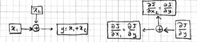
We model the unknown process using a prediction function, a parametric function that predicts the output of the process given its input. Here is an example:
\[\hat{y} = W x + b\]
Here $x$ is the model input, $\hat{y}$ is the model output, $W$ is a matrix of weights, and $b$ is a vector of biases. By adjusting the parameters of this model, i.e. the weights and the biases, we can make it compute any linear function of $x$.
"All models are wrong, but some models are useful." George Box famously said. We do not necessarily know that the system whose output we are trying to predict is governed by a linear relationship. All we know is a finite number of input-output examples in the training data:
\[\mathcal{D}=\{(x_1,y_1),\ldots,(x_N,y_N)\}\]
It is just that we have to start model building somewhere and the set of all linear functions is a good place to start for now.
A commonly used loss function in problems with numeric outputs is the squared error, i.e. the average squared difference between the actual output values and the ones predicted by the model. So our goal is to find model parameters that minimize the squared error:
\[\arg\min_{W,b} \frac{1}{N} \sum_{n=1}^N \| \hat{y}_n - y_n \|^2\]
Where $\hat{y}_n = W x_n + b$ denotes the output predicted by the model for the $n$ th example.
There are several methods to find the solution to the problem of minimizing squared error. Here we will present the stochastic gradient descent (SGD) method because it generalizes well to more complex models. In SGD, we take the training examples (individually or in groups), compute the gradient of the error for the current example(s) with respect to the parameters using the backpropagation algorithm, and move the parameters a small step in the direction that will decrease the error. First some notes on the math.
Partial derivatives
When we have a function with a scalar output, we can look at how its value changes in response to a small change in one of its inputs or parameters, holding the rest fixed. This is called a partial derivative. Let us consider the squared error for the $n$ th input as an example:
\[J = \| W x_n + b - y_n \|^2\]
So the partial derivative $\partial J / \partial w_{ij}$ would tell us how many units $J$ would move if we moved $w_{ij}$ in $W$ one unit (at least for small enough units). Here is a more graphical representation:
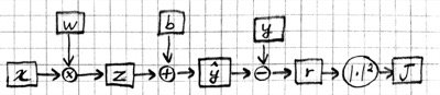
In this figure, it is easier to see that the machinery that generates $J$ has many "inputs". In particular we can talk about how $J$ is effected by changing parameters $W$ and $b$, as well as changing the input $x$, the model output $\hat{y}$, the desired output $y$, or intermediate values like $z$ or $r$. So partial derivatives like $\partial J / \partial x_i$ or $\partial J / \partial \hat{y}_j$ are fair game and tell us how $J$ would react in response to small changes in those quantities.
Chain rule and backpropagation
The chain rule allows us to calculate partial derivatives in terms of other partial derivatives, simplifying the overall computation. We will go over it in some detail as it forms the basis of the backpropagation algorithm. For now let us assume that each of the variables in the above example are scalars. We will start by looking at the effect of $r$ on $J$ and move backward from there. Basic calculus tells us that:
\[\begin{aligned} J &= r^2 \\ {\partial J}/{\partial r} &= 2r \end{aligned}\]
Thus, if $r=5$ and we decrease $r$ by a small $\epsilon$, the squared error $J$ will go down by $10\epsilon$. Now let's move back a step and look at $\hat{y}$:
\[\begin{aligned} r &= \hat{y} - y \\ {\partial r}/{\partial \hat{y}} &= 1 \end{aligned}\]
So how much effect will a small $\epsilon$ decrease in $\hat{y}$ have on $J$ when $r=5$? Well, when $\hat{y}$ goes down by $\epsilon$, so will $r$, which means $J$ will go down by $10\epsilon$ again. The chain rule expresses this idea:
\[\frac{\partial J}{\partial\hat{y}} = \frac{\partial J}{\partial r} \frac{\partial r}{\partial\hat{y}} = 2r\]
Going back further, we have:
\[\begin{aligned} \hat{y} &= z + b \\ {\partial \hat{y}}/{\partial b} &= 1 \\ {\partial \hat{y}}/{\partial z} &= 1 \end{aligned}\]
Which means $b$ and $z$ have the same effect on $J$ as $\hat{y}$ and $r$, i.e. decreasing them by $\epsilon$ will decrease $J$ by $2r\epsilon$ as well. Finally:
\[\begin{aligned} z &= w x \\ {\partial z}/{\partial x} &= w \\ {\partial z}/{\partial w} &= x \end{aligned}\]
This allows us to compute the effect of $w$ on $J$ in several steps: moving $w$ by $\epsilon$ will move $z$ by $x\epsilon$, $\hat{y}$ and $r$ will move exactly the same amount because their partials with $z$ are 1, and finally since $r$ moves by $x\epsilon$, $J$ will move by $2rx\epsilon$.
\[\frac{\partial J}{\partial w} = \frac{\partial J}{\partial r} \frac{\partial r}{\partial \hat{y}} \frac{\partial \hat{y}}{\partial z} \frac{\partial z}{\partial w} = 2rx\]
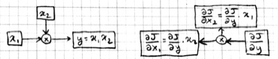
We can represent this process of computing partial derivatives as follows:
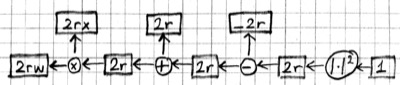
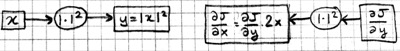
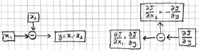
Note that we have the same number of boxes and operations, but all the arrows are reversed. Let us call this the backward pass, and the original computation in the previous picture the forward pass. Each box in this backward-pass picture represents the partial derivative for the corresponding box in the previous forward-pass picture. Most importantly, each computation is local: each operation takes the partial derivative of its output, and multiplies it with a factor that only depends on the original input/output values to compute the partial derivative of its input(s). In fact we can implement the forward and backward passes for the linear regression model using the following local operations:
This is basically the backpropagation algorithm in a nutshell, i.e. backpropagation can be viewed as the application of Leibniz' chain rule from 1660s to machine learning in 1980s.
Multiple dimensions
Let's look at the case where the input and output are not scalars but vectors. In particular assume that $x \in \mathbb{R}^D$ and $y \in \mathbb{R}^C$. This makes $W \in \mathbb{R}^{C\times D}$ a matrix and $z,b,\hat{y},r$ vectors in $\mathbb{R}^C$. During the forward pass, $z=Wx$ operation is now a matrix-vector product, the additions and subtractions are elementwise operations. The squared error $J=\|r\|^2=\sum r_i^2$ is still a scalar. For the backward pass we ask how much each element of these vectors or matrices effect $J$. Starting with $r$:
\[\begin{aligned} J &= \sum r_i^2 \\ {\partial J}/{\partial r_i} &= 2r_i \end{aligned}\]
We see that when $r$ is a vector, the partial derivative of each component is equal to twice that component. If we put these partial derivatives together in a vector, we obtain a gradient vector:
\[\nabla_r J \equiv \langle \frac{\partial J}{\partial r_1}, \cdots, \frac{\partial J}{\partial r_C} \rangle = \langle 2 r_1, \ldots, 2 r_C \rangle = 2\vec{r}\]
The addition, subtraction, and square norm operations work the same way as before except they act on each element. Moving back through the elementwise operations we see that:
\[\nabla_r J = \nabla_{\hat{y}} J = \nabla_b J = \nabla_z J = 2\vec{r}\]
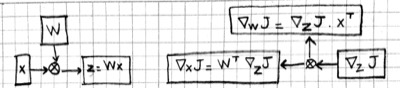
For the operation $z=Wx$, a little algebra will show you that:
\[\begin{aligned} \nabla_W J &= \nabla_z J \cdot x^T \\ \nabla_x J &= W^T \cdot \nabla_z J \end{aligned}\]
Note that the gradient of a variable has the same shape as the variable itself. In particular $\nabla_W J$ is a $C\times D$ matrix. Here is the graphical representation for matrix multiplication:
Multiple instances
We will typically process data multiple instances at a time for efficiency. Thus, the input $x$ will be a $D\times N$ matrix, and the output $y$ will be a $C\times N$ matrix, the $N$ columns representing $N$ different instances. Please verify to yourself that the forward and backward operations as described above handle this case without much change: the elementwise operations act on the elements of the matrices just like vectors, and the matrix multiplication and its gradient remains the same. Here is a picture of the forward and backward passes:
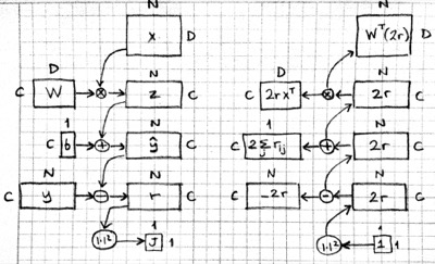
The only complication is at the addition of the bias vector. In the batch setting, we are adding $b\in\mathbb{R}^{C\times 1}$ to $z\in\mathbb{R}^{C\times N}$. This will be a broadcasting operation, i.e. the vector $b$ will be added to each column of the matrix $z$ to get $\hat{y}$. In the backward pass, we'll need to add the columns of $\nabla_{\hat{y}} J$ to get the gradient $\nabla_b J$.
Stochastic Gradient Descent
The gradients calculated by backprop, $\nabla_w J$ and $\nabla_b J$, tell us how much small changes in corresponding entries in $w$ and $b$ will effect the error (for the current example(s)). Small steps in the gradient direction will increase the error, steps in the opposite direction will decrease the error.
In fact, we can show that the gradient is the direction of steepest ascent. Consider a unit vector $v$ pointing in some arbitrary direction. The rate of change in this direction, $\nabla_v J$ (directional derivative), is given by the projection of $v$ onto the gradient, $\nabla J$, i.e. their dot product $\nabla J \cdot v$:
\[\nabla_v J = \frac{\partial J}{\partial x_1} v_1 + \frac{\partial J}{\partial x_2} v_2 + \cdots = \nabla J \cdot v\]
What direction maximizes this dot product? Recall that:
\[\nabla J \cdot v = | \nabla J |\,\, | v | \cos(\theta)\]
where $\theta$ is the angle between $v$ and the gradient vector. $\cos(\theta)$ is maximized when the two vectors point in the same direction. So if you are going to move a fixed (small) size step, the gradient direction gives you the biggest bang for the buck.
This suggests the following update rule:
\[w \leftarrow w - \nabla_w J\]
This is the basic idea behind Stochastic Gradient Descent (SGD): Go over the training set instance by instance (or minibatch by minibatch). Run the backpropagation algorithm to calculate the error gradients. Update the weights and biases in the opposite direction of these gradients. Rinse and repeat...
Housing Example
We will use the Boston Housing dataset from the UCI Machine Learning Repository to train a linear regression model using backprop and SGD. The dataset has housing related information for 506 neighborhoods in Boston from 1978. Each neighborhood has 14 attributes, the goal is to use the first 13, such as average number of rooms per house, or distance to employment centers, to predict the 14’th attribute: median dollar value of the houses.
First, we download and convert the data into Julia arrays. The Knet package provides some utilities for this:
using Knet
include(Knet.dir("data","housing.jl"))
x,y = housing()  # x is (13,506); y is (1,506)
Second, we implement our loss calculation in Julia. Personally I think callable objects are the most natural way to represent parametric functions. But you can use any coding style you wish as long as you can calculate a scalar loss from parameters and data.
struct Linear; w; b; end                  # new type that can be used as a function
(f::Linear)(x) = f.w * x .+ f.b           # prediction function if one argument
(f::Linear)(x,y) = mean(abs2, f(x) - y)   # loss function if two arguments
Now we can initialize a model, make some predictions, and calculate loss:
julia> model = Linear(zeros(1,13), zeros(1))
Linear([0.0 0.0 … 0.0 0.0], [0.0])

julia> pred = model(x)          # predictions for 506 instances
1×506 Array{Float64,2}:
 0.0   0.0   0.0   …  0.0   0.0   0.0

julia> y                        # not too close to real outputs
1×506 Array{Float64,2}:
 24.0  21.6  34.7  …  23.9  22.0  11.9

julia> loss = model(x,y)        # average loss for 506 instances
592.1469169960474
The loss gradients with respect to the model parameters can be computed manually as described above:
julia> r = (model(x) - y) / length(y)
1×506 Array{Float64,2}:
 -0.0474308  -0.0426877  -0.0685771  …  -0.0472332  -0.0434783  -0.0235178

julia> ∇w = 2r * x'
1×13 Array{Float64,2}:
 7.12844  -6.617  8.88016  -3.2174  …  8.60132  9.32187  -6.12163  13.5419

julia> ∇b = sum(2r)
-45.06561264822134
For larger models manual gradient calculation becomes impractical. The Knet package can calculate gradients automatically for us: (1) mark the parameters with the Param type, (2) apply the @diff macro to the loss calculation, (3) the grad function calculates the gradients:
julia> model = Linear(Param(zeros(1,13)), Param(zeros(1)))
Linear(P(Array{Float64,2}(1,13)), P(Array{Float64,1}(1)))

julia> loss = @diff model(x,y)
T(592.1469169960474)

julia> grad(loss, model.w)
1×13 Array{Float64,2}:
 7.12844  -6.617  8.88016  -3.2174  …  8.60132  9.32187  -6.12163  13.5419

julia> grad(loss, model.b)
1-element Array{Float64,1}:
 -45.06561264822134
We can use the gradients to train our model:
function sgdupdate(model, x, y)
    loss = @diff model(x, y)
    for p in params(model)
        p .-= 0.1 * grad(loss, p)
    end
    return value(loss)
end
Here is a plot of the loss value vs the number of updates:
julia> using Plots
julia> plot([sgdupdate(model,x,y) for i in 1:20])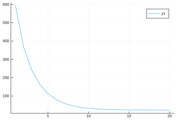
The new predictions are a lot closer to the actual outputs:
julia> [ model(x); y ]
2×506 Array{Float64,2}:
 30.4126  24.8121  30.7946  29.2931  …  27.6193  26.1515  21.9643
 24.0     21.6     34.7     33.4        23.9     22.0     11.9
Problems with SGD
Over the years, people have noted many subtle problems with the SGD algorithm and suggested improvements:
Step size: If the step sizes are too small, the SGD algorithm will take too long to converge. If they are too big it will overshoot the optimum and start to oscillate. So we scale the gradients with an adjustable parameter called the learning rate $\eta$:
$w \leftarrow w - \eta \nabla_w J$
Step direction: More importantly, it turns out the gradient (or its opposite) is often NOT the direction you want to go in order to minimize error. Let us illustrate with a simple picture:
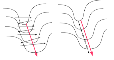
The figure on the left shows what would happen if you stood on one side of the long narrow valley and took the direction of steepest descent: this would point to the other side of the valley and you would end up moving back and forth between the two sides, instead of taking the gentle incline down as in the figure on the right. The direction across the valley has a high gradient but also a high curvature (second derivative) which means the descent will be sharp but short lived. On the other hand the direction following the bottom of the valley has a smaller gradient and low curvature, the descent will be slow but it will continue for a longer distance. Newton's method adjusts the direction taking into account the second derivative:
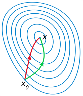
In this figure, the two axes are w1 and w2, two parameters of our network, and the contour plot represents the error with a minimum at x. If we start at x0, the Newton direction (in red) points almost towards the minimum, whereas the gradient (in green), perpendicular to the contours, points to the right.
Unfortunately Newton's direction is expensive to compute. However, it is also probably unnecessary for several reasons: (1) Newton gives us the ideal direction for second degree objective functions, which our objective function almost certainly is not, (2) The error function whose gradient backprop calculated is the error for the last minibatch/instance only, which at best is a very noisy approximation of the real error function, thus we shouldn't spend too much effort trying to get the direction exactly right.
So people have come up with various approximate methods to improve the step direction. Instead of multiplying each component of the gradient with the same learning rate, these methods scale them separately using their running average (momentum, Nesterov), or RMS (Adagrad, Rmsprop). Some even cap the gradients at an arbitrary upper limit (gradient clipping) to prevent instabilities.
You may wonder whether these methods still give us directions that consistently increase/decrease the objective function. If we do not insist on the maximum increase, any direction whose components have the same signs as the gradient vector is guaranteed to increase the function (for short enough steps). The reason is again given by the dot product $\nabla J \cdot v$. As long as these two vectors carry the same signs in the same components, the dot product, i.e. the rate of change along $v$, is guaranteed to be positive.
Minimize what? The final problem with gradient descent, other than not telling us the ideal step size or direction, is that it is not even minimizing the right objective! We want small error on never before seen test data, not just on the training data. The truth is, a sufficiently large model with a good optimization algorithm can get arbitrarily low error (down to the noise limit) on any finite training data (e.g. by just memorizing the answers). And it can typically do so in many different ways (typically many different local minima for training error in weight space exist). Some of those ways will generalize well to unseen data, some won't. And unseen data is (by definition) not seen, so how will we ever know which weight settings will do well on it?
There are at least three ways people deal with this problem: (1) Bayes tells us that we should use all possible models and weigh their answers by how well they do on training data (see Radford Neal's fbm), (2) New methods like dropout that add distortions and noise to inputs, activations, or weights during training seem to help generalization, (3) Pressuring the optimization to stay in one corner of the weight space (e.g. L1, L2, maxnorm regularization) helps generalization.
References
- UFLDL Tutorial, Linear Regression
- cs231n Optimization Notes
- cs229 Convex optimization overview, Part 2
- cs229 Linear algebra review and reference
- cs229 Review of probability theory
Notes
Supervised learning is also known as regression if the outputs are numeric and classification if they are discrete.
Linear regression is a regression model with a linear prediction function. Linear regression with a scalar input and output is called simple linear regression, if the input is a vector we have multiple linear regression, and if the output is a vector we have multivariate linear regression.